Inference about Models • umncvmstats

Inference about a correlation

correlation_inference(mpg ~ wt + hp, data = mtcars2)

response	variable	correlation	conf.low	conf.high	p.value
mpg	wt	−0.868	−0.934	−0.744	< 0.0001
mpg	hp	−0.78	−0.89	−0.59	< 0.0001
Pearson's product-moment correlation (two.sided), with 95% confidence intervals

Model Creation

This code works with most linear or logistic models; it also has special handling for models with a log-transformed response

Start by building the models in the usual way; here are three models. All have both a categorical and a continuous explanatory variable, and their interaction.

A linear model
A linear model with a log-transformed response
A logistic model

m1 <- lm(mpg ~ wt * cyl, data = mtcars2)
m1_log <- lm(log(mpg) ~ wt * cyl, data = mtcars2)
m2 <- glm(am ~ mpg * cyl, data = mtcars2, family=binomial)

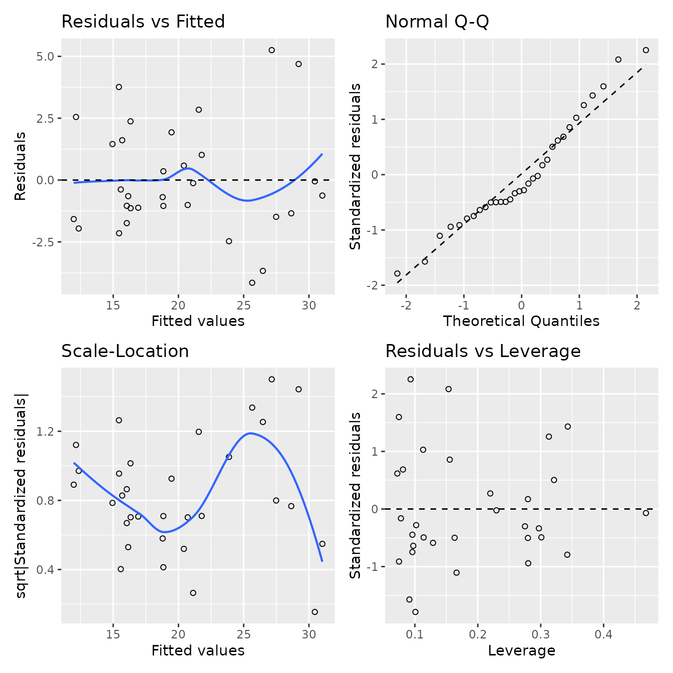
Model Diagnostics

diag_plots(m1)

ANOVA / Analysis of Deviance

model_anova(m1)

term	df	sumsq	meansq	F	p.value
mpg ~ wt * cyl
wt	1	118	118	19.7	0.0001
cyl	2	95.3	47.6	7.94	0.0020
wt:cyl	2	27.2	13.6	2.27	0.12
Residuals	26	156	6.00

model_anova(m1_log)

term	df	sumsq	meansq	F	p.value
log(mpg) ~ wt * cyl
wt	1	0.357	0.357	24.6	< 0.0001
cyl	2	0.173	0.0864	5.95	0.0075
wt:cyl	2	0.00603	0.00301	0.208	0.81
Residuals	26	0.378	0.0145

model_anova(m2)

term	df	chisq	p.value
(am = manual) ~ mpg * cyl
mpg	1	4.53	0.033
cyl	2	0.271	0.87
mpg:cyl	2	1.73	0.42

Model summary values

model_glance(m1)

df	r.squared	adj.r.squared	sigma	statistic	logLik	AIC	BIC	deviance	df.residual	nobs	p.value
mpg ~ wt * cyl
5	0.862	0.835	2.45	32.4	-70.7	155	166	156	26	32	< 0.0001

model_glance(m2)

null.deviance	df.null	logLik	AIC	BIC	deviance	df.residual	nobs
(am = manual) ~ mpg * cyl
43.2	31	-13.8	39.7	48.5	27.7	26	32

Model coefficients

combine_tests(
  model_coefs(m1),
  model_coefs(m1_log),
  model_coefs(m2))

	term	estimate	SE	statistic	p.value
mpg ~ wt * cyl	(Intercept)	39.6	3.2	12.4	< 0.0001
	wt	−5.6	1.4	-4.15	0.0003
	cyl6	−11.2	9.4	-1.19	0.24
	cyl8	−15.7	4.8	-3.24	0.0032
	wt:cyl6	2.9	3.1	0.920	0.37
	wt:cyl8	3.5	1.6	2.12	0.043
log(mpg) ~ wt * cyl	(Intercept)	3.75	0.16	23.9	< 0.0001
	wt	−0.212	0.067	-3.16	0.0039
	cyl6	−0.33	0.46	-0.710	0.48
	cyl8	−0.40	0.24	-1.67	0.11
	wt:cyl6	0.07	0.15	0.446	0.66
	wt:cyl8	0.048	0.080	0.596	0.56
(am = manual) ~ mpg * cyl	(Intercept)	−11.0	8.3	-1.33	0.18
	mpg	0.48	0.35	1.38	0.17
	cyl6	−9	18	-0.496	0.62
	cyl8	8.3	9.6	0.864	0.39
	mpg:cyl6	0.49	0.85	0.584	0.56
	mpg:cyl8	−0.42	0.47	-0.897	0.37

Model prediction intervals

model_predictions(m1, at=list(wt=c(2,3,4), cyl=c("4", "8")))

wt	cyl	prediction	predict.low	predict.high
mpg ~ wt * cyl
2.00	4	28.3	23.0	33.6
2.00	8	19.5	13.1	25.9
3.00	4	22.6	17.0	28.3
3.00	8	17.3	11.8	22.8
4.00	4	17.0	9.9	24.1
4.00	8	15.1	9.9	20.3
Prediction level used: 0.95

For log response models, model predictions and prediction intervals are automatically backtransformed.

model_predictions(m1_log, at=list(wt=c(2,3,4), cyl=c("4", "8")))

wt	cyl	prediction	predict.low	predict.high
log(mpg) ~ wt * cyl
2.00	4	28.0	21.5	36.3
2.00	8	20.7	15.1	28.3
3.00	4	22.6	17.2	29.8
3.00	8	17.5	13.4	23.0
4.00	4	18.3	12.9	26.0
4.00	8	14.9	11.5	19.2
Prediction level used: 0.95
Predictions are back-transformed from the log scale

Model means

For log response and logistic models, model means and confidence intervals are automatically backtransformed. That is, to the original scale from the log scale for log responses, and to the probability scale from the log-odds scale for logistic models. To see results on the log or logistic scale, use backtransform = FALSE.

Linear Model

model_means(m1, ~1)

1	emmean	SE	df	conf.low	conf.high
mpg ~ wt * cyl
overall	19.23	0.67	26	17.86	20.60
Results are averaged over the levels of: cyl
Confidence level used: 0.95

model_means(m1, ~cyl)

cyl	emmean	SE	df	conf.low	conf.high	cld.group
mpg ~ wt * cyl
8	16.81	0.96	26	14.85	18.78	a
6	19.46	0.97	26	17.48	21.45	ab
4	21.4	1.5	26	18.4	24.4	b
Confidence level used: 0.95
P value adjustment: tukey method for comparing a family of 3 estimates
significance level used: alpha = 0.05
NOTE: Results may be misleading due to involvement in interactions

pairwise_model_means(m1, ~cyl)

contrast	estimate	SE	df	conf.low	conf.high	t.ratio	p.value
mpg ~ wt * cyl
cyl4 - cyl6	1.9	1.8	26	−2.4	6.3	1.10	0.52
cyl4 - cyl8	4.6	1.8	26	0.2	8.9	2.62	0.037
cyl6 - cyl8	2.7	1.4	26	−0.7	6.0	1.95	0.15
Confidence level used: 0.95
Conf-level adjustment: tukey method for comparing a family of 3 estimates
P value adjustment: tukey method for comparing a family of 3 estimates
NOTE: Results may be misleading due to involvement in interactions

model_means(m1, ~cyl | wt, at=list(wt=c(2,3,4)))

	cyl	emmean	SE	df	conf.low	conf.high	cld.group
mpg ~ wt * cyl
wt = 2	8	19.5	1.9	26	15.6	23.4	a
	6	22.8	3.3	26	16.1	29.6	ab
	4	28.28	0.83	26	26.56	29.99	b
wt = 3	8	17.3	1.1	26	15.0	19.6	a
	6	20.07	0.98	26	18.05	22.09	ab
	4	22.6	1.2	26	20.1	25.1	b
wt = 4	8	15.10	0.65	26	13.75	16.44	a
	4	17.0	2.4	26	12.0	22.0	a
	6	17.3	2.6	26	11.9	22.7	a
Confidence level used: 0.95
P value adjustment: tukey method for comparing a family of 3 estimates
significance level used: alpha = 0.05

pairwise_model_means(m1, ~cyl | wt, at=list(wt=c(2,3,4)))

	contrast	estimate	SE	df	conf.low	conf.high	t.ratio	p.value
mpg ~ wt * cyl
wt = 2	cyl4 - cyl6	5.4	3.4	26	−3.0	13.8	1.61	0.26
	cyl4 - cyl8	8.8	2.1	26	3.6	14.0	4.23	0.0007
	cyl6 - cyl8	3.4	3.8	26	−6.0	12.8	0.890	0.65
wt = 3	cyl4 - cyl6	2.6	1.6	26	−1.3	6.5	1.64	0.25
	cyl4 - cyl8	5.3	1.6	26	1.2	9.4	3.24	0.0088
	cyl6 - cyl8	2.8	1.5	26	−0.9	6.5	1.88	0.17
wt = 4	cyl4 - cyl6	−0.3	3.6	26	−9.3	8.6	-0.0848	1.0
	cyl4 - cyl8	1.9	2.5	26	−4.4	8.2	0.745	0.74
	cyl6 - cyl8	2.2	2.7	26	−4.6	9.0	0.804	0.70
Confidence level used: 0.95
Conf-level adjustment: tukey method for comparing a family of 3 estimates
P value adjustment: tukey method for comparing a family of 3 estimates

Linear Model, with log response

model_means(m1_log, ~cyl)

cyl	response	SE	df	conf.low	conf.high	cld.group
log(mpg) ~ wt * cyl
8	16.92	0.80	26	15.36	18.64	a
6	19.42	0.92	26	17.61	21.41	ab
4	21.6	1.6	26	18.6	25.1	b
Confidence level used: 0.95
Intervals are back-transformed from the log scale
P value adjustment: tukey method for comparing a family of 3 estimates
Tests are performed on the log scale
significance level used: alpha = 0.05
NOTE: Results may be misleading due to involvement in interactions

pairwise_model_means(m1_log, ~cyl)

contrast	ratio	SE	df	conf.low	conf.high	null	t.ratio	p.value
log(mpg) ~ wt * cyl
cyl4 / cyl6	1.113	0.096	26	0.898	1.380	1.00	1.24	0.44
cyl4 / cyl8	1.28	0.11	26	1.03	1.58	1.00	2.84	0.023
cyl6 / cyl8	1.148	0.077	26	0.972	1.355	1.00	2.05	0.12
Confidence level used: 0.95
Conf-level adjustment: tukey method for comparing a family of 3 estimates
Intervals are back-transformed from the log scale
P value adjustment: tukey method for comparing a family of 3 estimates
Tests are performed on the log scale
NOTE: Results may be misleading due to involvement in interactions

pairwise_model_means(m1_log, ~cyl, backtransform = FALSE)

contrast	estimate	SE	df	conf.low	conf.high	t.ratio	p.value
log(mpg) ~ wt * cyl
cyl4 - cyl6	0.107	0.086	26	−0.108	0.322	1.24	0.44
cyl4 - cyl8	0.245	0.086	26	0.031	0.459	2.84	0.023
cyl6 - cyl8	0.138	0.067	26	−0.029	0.304	2.05	0.12
Results are given on the log (not the response) scale.
Confidence level used: 0.95
Conf-level adjustment: tukey method for comparing a family of 3 estimates
P value adjustment: tukey method for comparing a family of 3 estimates
NOTE: Results may be misleading due to involvement in interactions

model_means(m1_log, ~cyl, backtransform = FALSE)

cyl	emmean	SE	df	conf.low	conf.high	cld.group
log(mpg) ~ wt * cyl
8	2.828	0.047	26	2.732	2.925	a
6	2.966	0.048	26	2.868	3.064	ab
4	3.073	0.072	26	2.925	3.221	b
Results are given on the log (not the response) scale.
Confidence level used: 0.95
P value adjustment: tukey method for comparing a family of 3 estimates
significance level used: alpha = 0.05
NOTE: Results may be misleading due to involvement in interactions

Logistic Model

model_means(m2, ~cyl)

cyl	prob	SE	conf.low	conf.high	cld.group
(am = manual) ~ mpg * cyl
8	0.18	0.25	0.01	0.86	a
4	0.21	0.24	0.01	0.83	a
6	0.48	0.23	0.13	0.84	a
Confidence level used: 0.95
Intervals are back-transformed from the logit scale
P value adjustment: tukey method for comparing a family of 3 estimates
Tests are performed on the log odds ratio scale
significance level used: alpha = 0.05
NOTE: Results may be misleading due to involvement in interactions

pairwise_model_means(m2, ~cyl)

contrast	odds.ratio	SE	conf.low	conf.high	null	z.ratio	p.value
(am = manual) ~ mpg * cyl
cyl4 / cyl6	0.29	0.51	0.01	16.85	1.00	-0.709	0.76
cyl4 / cyl8	1.2	2.7	0.0	228.5	1.00	0.0805	1.0
cyl6 / cyl8	4.1	7.8	0.0	362.4	1.00	0.734	0.74
Confidence level used: 0.95
Conf-level adjustment: tukey method for comparing a family of 3 estimates
Intervals are back-transformed from the log odds ratio scale
P value adjustment: tukey method for comparing a family of 3 estimates
Tests are performed on the log odds ratio scale
NOTE: Results may be misleading due to involvement in interactions

model_means(m2, ~cyl, backtransform=FALSE)

cyl	emmean	SE	conf.low	conf.high	cld.group
(am = manual) ~ mpg * cyl
8	−1.5	1.7	−4.8	1.8	a
4	−1.3	1.5	−4.2	1.6	a
6	−0.10	0.90	−1.87	1.67	a
Results are given on the logit (not the response) scale.
Confidence level used: 0.95
Results are given on the log odds ratio (not the response) scale.
P value adjustment: tukey method for comparing a family of 3 estimates
significance level used: alpha = 0.05
NOTE: Results may be misleading due to involvement in interactions

pairwise_model_means(m2, ~cyl, backtransform=FALSE)

contrast	estimate	SE	conf.low	conf.high	z.ratio	p.value
(am = manual) ~ mpg * cyl
cyl4 - cyl6	−1.2	1.7	−5.3	2.8	-0.709	0.76
cyl4 - cyl8	0.2	2.2	−5.1	5.4	0.0805	1.0
cyl6 - cyl8	1.4	1.9	−3.1	5.9	0.734	0.74
Results are given on the log odds ratio (not the response) scale.
Confidence level used: 0.95
Conf-level adjustment: tukey method for comparing a family of 3 estimates
P value adjustment: tukey method for comparing a family of 3 estimates
NOTE: Results may be misleading due to involvement in interactions

Model slopes

For continuous explanatory variables, the slopes can be obtained and compared in a similar way.

model_slopes(m1, wt~1)

1	wt.trend	SE	df	conf.low	conf.high	t.ratio	p.value
mpg ~ wt * cyl
overall	−3.5	1.1	26	−5.8	−1.3	-3.27	0.0030
Results are averaged over the levels of: cyl
Confidence level used: 0.95

model_slopes(m1, wt~cyl)

cyl	wt.trend	SE	df	conf.low	conf.high	t.ratio	p.value	cld.group
mpg ~ wt * cyl
4	−5.6	1.4	26	−8.4	−2.9	-4.15	0.0003	a
6	−2.8	2.8	26	−8.5	3.0	-0.991	0.33	a
8	−2.19	0.89	26	−4.03	−0.35	-2.45	0.021	a
Confidence level used: 0.95
P value adjustment: tukey method for comparing a family of 3 estimates
significance level used: alpha = 0.05

pairwise_model_slopes(m1, wt~cyl)

contrast	estimate	SE	df	conf.low	conf.high	t.ratio	p.value
mpg ~ wt * cyl
cyl4 - cyl6	−2.9	3.1	26	−10.6	4.9	-0.920	0.63
cyl4 - cyl8	−3.5	1.6	26	−7.5	0.6	-2.12	0.10
cyl6 - cyl8	−0.6	2.9	26	−7.9	6.7	-0.200	0.98
Confidence level used: 0.95
Conf-level adjustment: tukey method for comparing a family of 3 estimates
P value adjustment: tukey method for comparing a family of 3 estimates

For log-response or logistic models, no back-transformation is done.

model_slopes(m1_log, wt~cyl)

cyl	wt.trend	SE	df	conf.low	conf.high	t.ratio	p.value	cld.group
log(mpg) ~ wt * cyl
4	−0.212	0.067	26	−0.349	−0.074	-3.16	0.0039	a
8	−0.164	0.044	26	−0.255	−0.074	-3.73	0.0009	a
6	−0.14	0.14	26	−0.43	0.14	-1.04	0.31	a
Confidence level used: 0.95
P value adjustment: tukey method for comparing a family of 3 estimates
significance level used: alpha = 0.05

model_slopes(m2, mpg~cyl)

cyl	mpg.trend	SE	conf.low	conf.high	z.ratio	p.value	cld.group
(am = manual) ~ mpg * cyl
8	0.06	0.32	−0.56	0.68	0.185	0.85	a
4	0.48	0.35	−0.20	1.17	1.38	0.17	a
6	0.98	0.77	−0.53	2.49	1.27	0.21	a
Confidence level used: 0.95
P value adjustment: tukey method for comparing a family of 3 estimates
significance level used: alpha = 0.05